Interpreting structure and regolith thickness in an orogenic gold prospect from detailed gravity data using VPmg inversion software

Mapping the thickness of regolith developed over an orogenic gold project area can often provide clues to the location of structures and strongly altered zones, as these may be associated with development of a thicker weathering profile. Obtaining this information from drilling alone is expensive. Detailed gravity measurements provide one means of imaging variations in the thickness of the low density regolith overlying higher density fresh rock. This information can then be used for targeting and interpretation of geochemical data.

Detailed gravity data from an African gold exploration project were studied. Estimating the average density of the regolith layer – a necessary precursor to gravity data reduction and to modeling the response of a variable thickness regolith – was approached in two ways: linear regression of the Free Air Anomaly (FAA) versus Bouguer correction at unit density, and forward modeling the FAA using a range of terrain density values to find the one producing the best fit to observed gravity data. These density estimates, together with specific gravity measurements on drill core, were used as parameters in an inverse model recovered from the gravity data, defining the variable thickness of a constant density regolith layer overlying a denser basement. The resultant image of the depth to base of weathering contains a set of elongate depressions that have a strong association with known mineralization and gradient array IP anomalies possibly caused by sulphide in mineralized rock.

Introduction

Seko base saprolite RL

Modeling the gravity response of a variable thickness low-density layer overlying dense basement rocks provides a useful method for imaging variations in the thickness of the weathered layer. These weathered layer thickness variations often reflect hydrothermal alteration, changes in porosity related to structural fabric and lithology that are relevant to exploration targeting. The information can be especially useful in areas where the basement rocks are magnetically “flat” – the regolith gravity response may be the only cheaply available and helpful geophysical mapping tool.

In itself, this kind of regolith imaging can be useful for interpretation of geochemical datasets. Transforming the gravity data into a map of a geological surface makes them easier to integrate with other datasets.

The program VPmg provides a means of recovering an inverse model composed of homogeneous or inhomogeneous layers characterized by density or magnetic properties (induced or remanent magnetization). In its simplest implementation – an upper layer forming a flat contact with a homogeneous basement – this type of model can be useful for estimating average terrain density used in reduction of gravity data. This forms a basis for developing a more complex layered model, as demonstrated in this article.

Geology

Basement rocks within the survey area consist mainly of sedimentary rock (greywacke, siltstone, shale), intermediate volcanics and felsic intrusives, intruded by dolerite dykes. Gold mineralization occurs in several NNW-trending shear zones that have been located through auger drilling and gradient array induced polarization surveys. Outcrop of fresh rock is virtually non-existent, and prospecting for gold has been performed using auger drilling of the weathered rock.

The area has been subject to lateritic weathering, a chemical process occurring in tropical climates where acidic groundwater attacks the primary minerals, removing silica, alkalis and alkaline earths, resulting in residual or relative enrichment of iron and frequently of aluminium. The resulting regolith profile (Figure 1) in the area of interest is dominated by the saprolite layers, where the primary rocks are variably kaolinized but a relict portion of the original texture may be recognized. These grade downwards into saprock, where cores of unaltered rock are present, overlying fresh rock. We shall see below that there is a strong density contrast between the saprolite and fresh rock, which dominates the gravity response.

F2.large — **Figure 1**. Laterite weathering profile. Components of this profile may be more or less developed, depending on the weathering history of the area, and may be modified by subsequent weathering events.

Gravity survey

Seko DEM with stations — **Figure 2.** Colorshaded DEM image and station locations. The DEM was derived by gridding gravity station elevations.

Gravity and DGPS measurements were acquired on east-west traverses, mainly at 200m line spacing and 100m station spacing along-line (Figure 2). Station elevations within the survey area ranged from 150 m to 219 m. The terrain is typical of laterite incised by drainage and outcrop is nonexistent.

The gravity response is subdued: the simple Bouguer anomaly (1.90 g/cc) range is only 2.81 mGal and the standard deviation 0.56 mGal. The range of Bouguer corrections at this density value is 5.47 mGal, with a mean of 14.31 mGal and standard deviation 0.99 mGal. In view of the large magnitude of these corrections in comparison to the range of Bouguer anomaly values, determining the appropriate Bouguer slab density is critical to deriving useful data from the reduction process.

Data reduction

The simple Bouguer anomaly (or complete Bouguer anomaly if terrain corrections are applied) is the end-product of the gravity data reduction and correction process, wherein the meter drift, Earth tide, theoretical ellipsoid acceleration due to gravity, free air correction and Bouguer slab correction are removed from the data. The Bouguer correction is the contribution to the gravity response of an idealized infinite homogeneous slab of material lying between each station and a given height datum (commonly sea level). Removal of the Bouguer slab response from the Free Air Anomaly yields the “Bouguer anomaly”, which is the response of density inhomogeneities within the Earth – i.e. departures from the Bouguer slab density, which is the average density of the terrain in the survey area.

If the Bouguer slab density is not correctly estimated, the Bouguer anomaly values will contain a positive or negative residual component of the slab response, leading to interpretation problems. Several methods, surveyed by Yamamoto (1999), have been devised to estimate the Bouguer slab density directly from the gravity and height data, and these results should be evaluated against hand sample physical property measurements and ranges of possible values based on the geology and tabulations of average density values for various rock types.

A commonly used and effective method for estimating Bouguer slab density involves transforming the following expression for the Bouguer anomaly ${ g }_{ B }$ in terms of the Free Air Anomaly ${ g }_{ fa }$ and the Bouguer correction ${ \delta }_{ { g }_{ B } }$

${ g }_{ B }={ g }_{ fa }-{ \delta }_{ { g }_{ B } }={ g }_{ fa }-0.0419088{ \rho }_{ B }h$

by considering the Bouguer anomaly ${ g }_{ B }$ value to be equivalent to a small error term $\varepsilon$ (valid in cases such as this, where the Bouguer anomalies are small) and rearranging so that

${ g }_{ fa }={ \delta }_{ { g }_{ B } }+\varepsilon =0.0419088{ \rho }_{ B }h+\varepsilon$

i.e. the Bouguer slab density ${ \rho }_{ B }$ is the slope of a linear regression of Free Air Anomaly ${ g }_{ fa }$ values against scaled height values $0.0419088h$ (which are the Bouguer corrections with ${ \rho }_{ B }=1$ ).

Applying this method to the survey data (Figure 3) gives an estimated Bouguer slab density of 2.02 g/cc. Note that this is well below the average for crustal rocks (2.67 g/cc), so blindly choosing that number would lead to serious error.

Parasnis method — Figure 3. Estimation of Bouguer slab density by linear regression of the Free Air Anomaly values against Bouguer correction values at 1 g/cc. The estimate of 2.02 g/cc is higher than typical specific gravity measurements on saprolite drill core specimens, but these are a very limited sample of near-surface rocks in the total survey area.

Seko Bouguer anomaly 2_00 — **Figure 4.** Colorshaded image of Bouguer anomaly (2.00 g/cc)

The Bouguer anomaly (2.00 g/cc) image (Figure 4) appears to be generally uncorrelated with the elevation image in Figure 1 above, giving us confidence that the statistically-derived Bouguer slab density value is reasonable. However, some of the narrow valleys have associated lows in the Bouguer anomaly image, possibly resulting from terrain effects or errors in the terrain density estimate.

An alternative method for estimating the Bouguer slab density, which incorporates terrain effects and allows for different density values to be applied in regions known to have significantly different geology (e.g. granite batholiths vs shale-dominated sedimentary sequences), involves comparing the observed Free Air Anomaly with values calculated using a simple model of a homogeneous upper layer in planar contact with a homogenous basement.

The modeling program VPmg was used to calculate the Free Air Anomaly at each station for a range of different model terrain densities, and the Root Mean Square (RMS) misfit between these calculated values and the observed data was graphed against the corresponding density value (Figure 5). The best-fitting data were calculated using a terrain density of 1.90 g/cc, which is close to the value estimated statistically from the gravity data above. The RMS misfit (0.52 mGal) is actually less than the standard deviation of the Bouguer anomaly values, so the simple model of a homogeneous layer overlying a denser basement is a good first-order approximation to the actual density structure of the Earth in this area. Not surprisingly, the residual gravity response estimated by subtracting this theoretical model response from the observed Free Air Anomaly values looks very similar to the Bouguer anomaly image in Figure 4 above.

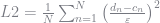
Misfit vs density — **Figure 5.** Data misfit versus model density. The best-fitting density value of 1.90 g/cc is close to the value (2.02 g/cc) statistically estimated from the gravity data.

Regolith densities

Drill core specific gravity measurements over a thick intersection of regolith (all within the upper and lower saprolite zones) are available from one hole. The length-weighted average value of specific gravity for the entire saprolite interval is 1.51, which happens to equal the raw average and median. The standard deviation is 0.07, and the range 0.26 (1.35 to 1.61). The density of saprolite is a good starting point for modeling the regolith as a whole in this instance: logging codes in the drilling database consist mainly of upper saprolite (51%) and lower saprolite (11%) while the upper (massive laterite 4%, pisolitic laterite 2%) and lower (saprock 5%) parts of the profile were intersected over a lesser proportion of intervals. This is admittedly a crude way of looking at the geology, but the dominance of saprolite in the drilled laterite profile is clear.

This average density estimate (1.51 g/cc) is significantly lower than the regolith density estimates established from the gravity data (1.90 – 2.00 g/cc). However, this individual drill hole may not be truly representative of the regolith densities across the entire survey area, and it should be noted that the ‘contact’ between regolith and fresh rock is gradational, rather than a sharp 1.50 to 2.80 g/cc density transition. These issues highlight the need to consider a range of possible density values when modeling the gravity data.

Basement densities

Limited basement drill core sampling (2 holes) with specific gravity measurements is available in the survey area. The basement is known to consist mainly of greywacke and shale, with some dolerite dykes. The histogram of drill core s.g. measurements (Figure 6) reflects these rock types. Including all rock types intersected by the holes, the mean specific gravity is 2.77 with standard deviation 0.09 – i.e. a fairly narrow spread of densities. Attempting to recover fairly subtle (±0.2 g/cc) density variations within the basement in the presence of a variable regolith profile having a contrast of about 0.90 g/cc relative to average basement density using gravity data alone is a tall order without blanket a priori information on regolith thickness. A more realistic objective would be recovering regolith thickness and making the assumption of a uniform basement density, recognizing that more strongly altered basement is likely to coincide with deeper weathering, particularly where the alteration assemblage includes significant sulphide content.

Histogram of densities — **Figure 6.** Histogram of drill core specific gravity measurements. Excluding the measurements on dolerite samples, the length-weighted mean specific gravity of all other rock types intersected by the two holes was 2.75

Homogenous layer inversion

Having established reasonable estimates of regolith and fresh rock densities, the model of regolith thickness (assuming homogeneous density in both layers) can be recovered from the gravity data using the inversion program VPmg.

Inversion is a computational process of finding a set of model parameters $m$ , given a set of observed data $d$ such that

$d=G(m)$

where $G$ is an operator that describes the relationship between model parameters and the geophysical response. The algorithm solves this problem approximately, such that an objective function describing the misfit between observed and calculated data is minimized. A commonly used objective function is the chi-squared data norm $L2$ defined as

$L2=\frac { 1 }{ N } \sum _{ n=1 }^{ N }{ { \left( \frac { { d }_{ n }-{ c }_{ n } }{ \varepsilon } \right) }^{ 2 } }$

where $d$ are the observed data, $c$ are the data calculated by applying the operator $G$ to the model parameters $m$ , and $\varepsilon$ is the assigned uncertainty, reflecting the estimated level of error in the observations.

Geological structures can be parameterized in different ways. For instance, the subsurface can be discretized into a set of cubic cells, each with its own uniform density, so that the set of densities forms the model parameters $m$ .

VPmg (which stands for “Vertical Prism magnetic gravity”) was written by Peter Fullagar and is marketed by Mira Geoscience. The program models density and magnetic property distributions using a set of vertical prisms that can be subdivided into layers. These layers form “lithologies” with common properties, so the properties of a group of prisms can be altered en masse. The dimensions of the cells within each vertical prism adapt to the topography and the thickness of the geological unit in the model (Figure 7). The program and general modeling approach is described in papers by Fullagar & Pears (2007) and Fullagar et al (2000, 2004, 2008).

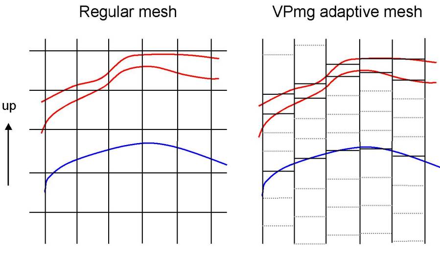
VPem3D_documentation_v3 — **Figure 7.** Schematic model sections illustrating the differences between a conventional
regular mesh (left) and the deforming mesh implemented in VPem3D. Vertical cell
dimensions are arbitrary, as required to best represent the geology. Horizontal cell
boundaries snap to geological contacts (coloured) in the VPem3D mesh, whereas all
boundaries are artificial in the regular mesh. Units can be sub-celled to permit internal
property variations. Sub-cell boundaries are dotted in the RH panel.

Seko base saprolite RL — **Figure 8.** Colorshaded image of base regolith elevation with gradient array IP chargeability peaks (blue squares). Many of the chargeable (sulphide-bearing?) trends defined by the IP are located within depressions in the base of weathering. Several of these coincident features are also associated with elevated gold in auger sampling. The outline of the IP survey is shown in light blue.

An inversion was run using a starting model consisting of regolith (1.90 g/cc) with basal contact at 145m elevation, overlying a homogeneous basement (2.80 g/cc). Only the elevation of the basal contact of the regolith in each model cell was allowed to vary. The inversion recovered a model producing an excellent fit to the observed data. The image of base regolith elevation (Figure 8) defines several discrete elongate zones in which the depth of weathering is greater than the surrounds, and these tend to coincide with elevated chargeability responses in gradient array IP data, which are also associated with gold anomalies in auger and aircore drilling. Some of the depressions in the base of weathering are consistent with drilling information (Figure 9). However, more work is required to refine the model, possibly including variations of the assumed density values.

Section_with_VPmg_model_anno — **Figure 9.** Drill section including base of weathering extracted from the geophysical model. The depression in the base of weathering defined by the density contrast in the model coincides with gold anomalism in aircore drilling of the saprolite. The geophysical model is broadly consistent with geological logging – both define a depression in the base of weathering.

The model is imperfect; east-west ridges corresponding to survey line locations are evident in the base of weathering surface, and these are due to greater sensitivity of the calculated response to these cells close to the readings compared to more distance model cells. The cells with lesser sensitivity tend not to be adjusted by the inversion to the same degree as the ones beneath the survey stations. A model with larger cells does not suffer from these artifacts to the same degree, but also has far lower spatial resolution. This model with 50m cells represents an attempt to squeeze maximum resolution from the model and the artifacts are a trade-off.

Compared to the colorshaded image of Bouguer gravity in Figure 4 above, the locations of depressions in the base of weathering are much more clearly defined in the model image in Figure 8.

Next steps

If some a priori information on depth to base of weathering were available across the entire survey area, this could be used as a constraint upon the homogeneous layer inversion discussed above, improving its accuracy. In all likelihood, density variations within the basement could then be recovered from the model, rather than fitting all of the variation in the data by varying the regolith thickness alone, as in the case discussed above. Unfortunately, drilling that penetrates the base of weathering is restricted to narrow zones where auger geochemistry has generated targets. The areas we are most interested in, by definition, have not yet been drilled. Techniques such as passive seismic or airborne EM may provide the needed information on variations in regolith thickness across wide enough areas to be useful.

Conclusion

The ability to forward model the effects of simple homogeneous terrain models at different densities allows us to find an average terrain density suitable for gravity data reduction. The calculated free air anomaly derived from this optimal model can be subtracted from the observed data to yield a residual gravity anomaly that incorporates both Bouguer slab and terrain corrections.

Inversion of gravity data from the subject orogenic gold project area has defined elongate zones of probable deeper weathering and/or more intense alteration, some of which correspond to structures that have already been drilled and found to be gold-bearing. Many of these zones coincide with elevated IP responses, which may be indicative of sulphide minerals in the alteration assemblage.

A potentially profitable area for further work involves using a priori models of transported and/or weathered material thickness to strip the gravity response of these layers from observed data, revealing the response component caused by basement structures.

References

Fullagar, P.K. and Pears, G.A.,2007, Towards geologically realistic inversion, in Proceedings of Exploration 07: Fifth Decennial International Conference on Mineral Exploration, Toronto.

Fullagar, P.K., Hughes, N., and Paine, J.,2000, Drilling-constrained 3D gravity interpretation, Exploration Geophysics, v. 31, p. 17-23.

Fullagar, P.K., Pears, G.A., Hutton, D., and Thompson, A.,2004, 3D gravity and aeromagnetic inversion, Pilbara region, W.A., Exploration Geophysics, v. 35, p. 142-146.

Fullagar, P.K., Pears, G.A., and McMonnies, B.,2008, Constrained inversion of geological surfaces – pushing the boundaries, The Leading Edge, v. 27, p. 98-105.

Yamamoto, A., 1999, Estimating the optimum reduction density for gravity anomaly: a theoretical overview: Jour. Fac. Sci., Hokkaido Univ., Ser. VII (Geophysics), Vol. 11, No.3, p577-599.